九、机器学习 Scikit-learn

9.1 SVM 分类

最终得到的决策函数为：f(x)=wTx+b。其中：

• w = coef_
• b = intercept_

import numpy as np
import pandas as pd
import matplotlib.pyplot as plt
from sklearn import svm

# 正类
p = np.random.normal(2, 1, (200, 2))
# 负类
f = np.random.normal(0, 1, (200, 2))
# 转为dataframe
df_p = pd.DataFrame(p, columns=list('XY'))
df_p['Z'] = 1
df_f = pd.DataFrame(f, columns=list('XY'))
df_f['Z'] = 0
# 合并f和p
con = pd.concat([df_p, df_f], axis=0)
# 重置索引 0-199 0-199 --> 0-399
con.reset_index(inplace=True, drop=True)

# 区分测试集、训练集
test_num = 150
trainData = con[0:-test_num] # 训练集必须包含2个及以上分类
testData = con[-test_num:]

# 选择训练集特征和标签
X = trainData[['X','Y']]
Z = trainData['Z']
X_test = testData[['X','Y']]
Z_test = testData['Z']
# SCV分类器
clf = svm.SVC(kernel='linear')
# 训练
clf.fit(X,Z)
# 得分
clf.score(X,Z)

print(f'系数：{clf.coef_}, {clf.intercept_}')
print(f'score:{clf.score(X_test,Z_test)}')

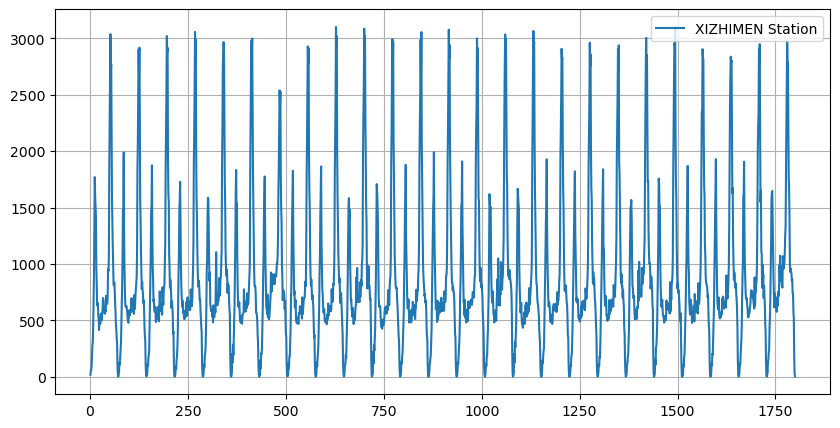
9.2 随机森林回归

import pandas as pd
import matplotlib.pyplot as plt
from sklearn.ensemble import RandomForestRegressor

# 读取文件
df = pd.read_csv('./scikit-learn/xizhimen.csv', encoding='gbk', parse_dates=True)
# 画图
plt.figure(figsize=(10,5))
plt.grid(True)
plt.plot(df.iloc[:,0], df.iloc[:,1], label="XIZHIMEN Station")
plt.legend()
plt.show()

# 新增前一天客流数据
df['pre_Date_flow'] = df.loc[:,['p_flow']].shift(1)
# 新增前5日平均客流数据
df['mean5'] = df.loc[:,['p_flow']].rolling(5).mean()
# 新增前10日平均客流数据
df['mean10'] = df.loc[:,['p_flow']].rolling(10).mean()
# 删除存在NaN的行
df.dropna(inplace=True)

X = df[['pre_Date_flow','mean5','mean10']]
Y = df['p_flow']
# 更改索引
X.index = range(X.shape[0])
# display(X)
# 设置训练集和测试集
num = int(X.shape[0] * 0.8)
X_train, X_test = X[:num], X[num:]
Y_train, Y_test = Y[:num], Y[num:]

# 预测 n_estimators为树的数量
rfr = RandomForestRegressor(n_estimators=15)
rfr.fit(X_train,Y_train)
score = rfr.score(X_test,Y_test)
res = rfr.predict(X_test)

# 画图
plt.figure(figsize=[15,5])
plt.title('The res of prediction')
plt.plot(Y_test.ravel(), label='real') # 扁平化Y_test，处理序号问题
plt.plot(res, label='predict')
plt.legend()
plt.show()

print(f'score: {score}')

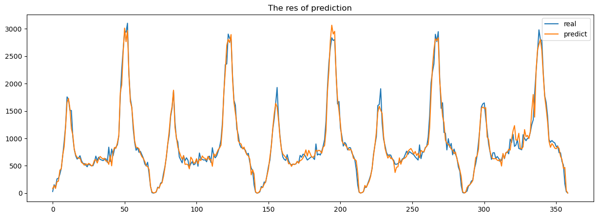
score: 0.9758139051758481

9.3 K-means 聚类

import matplotlib.pyplot as plt
import pandas as pd
from sklearn.cluster import KMeans
from sklearn import metrics

df = pd.read_csv('./scikit-learn/in_15min.csv',encoding='gbk')
df.dropna(inplace=True)
df.drop('Station_name',axis=1,inplace=True)

# 肘方法看K值（肘的位置，就是预估的分类树）
d=[]
for i in range(1,16):
    km = KMeans(n_clusters=i, init='k-means++', n_init=10, max_iter=300, random_state=0)
    km.fit(df)
    d.append(km.inertia_) # 记录簇内误差平方和

plt.plot(d, marker='o')
plt.xlabel('number of clusters')
plt.ylabel('distortions')
plt.show()

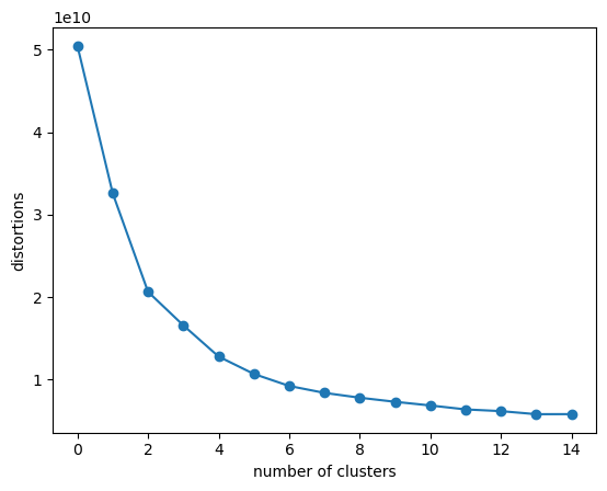
显然，肘部位即 k 是 6 或 7。

model_kmeans = KMeans(n_clusters=6, random_state=0)
model_kmeans.fit(df)

yPre = model_kmeans.predict(df)
print(yPre+1)

# 评价指标
silhouette_s = metrics.silhouette_score(df, yPre, metric = 'euclidean') # 欧氏距离计算样本间的距离
calinski_harabaz_s = metrics.calinski_harabasz_score(x_data, yPre)

print(f'轮廓系数：{silhouette_s}, 得分：{calinski_harabaz_s}')

[4 3 3 3 3 3 5 5 5 5 5 2 2 1 1 5 2 2 2 6 6 2 3 1 3 3 3 1 3 3 1 3 1 3 6 5 2
 3 5 1 1 2 5 6 2 6 5 5 5 2 3 1 1 1 1 1 3 1 1 3 3 3 3 3 2 3 1 5 1 5 1 5 5 5
 5 2 2 5 1 1 3 3 1 1 1 1 1 1 1 1 1 3 1 1 4 3 3 1 5 5 5 1 5 5 5 5 2 5 5 3 4
 3 4 4 3 1 5 5 5 1 5 2 2 5 3 3 3 3 3 3 3 1 3 1 1 1 2 1 3 5 1 1 1 5 1 2 5 1
 1 1 1 1 1 1 1 1 5 1 1 5 1 1 3 1 3 4 4 1 1 3 1 1 1 1 1 1 1 3 1 1 1 5 1 1 1
 1 1 3 5 1 1 5 5 5 1 1 1 1 3 1 1 3 3 1 3 1 4 3 3 2 2 1 2 2 5 3 5 5 5 2 2 5
 2 5 1 5 3 4 4 6 3 2 5 1 1 1 1 1 1 1 1 1 1 1 2 5 5 5 5 1 1 1 1 1 1 1 1 1 1
 1 1 1 1 1 3 1 3 1 3 3 1 1 1 1 1 1]
轮廓系数：0.3834164912580164, 得分：201.18789879013613

1. silhouette_score：轮廓系数（Silhouette Coefficient） 作用：评价聚类的紧密度和分离度。值的范围在 [-1, 1] 之间。 + 越接近 1，说明每个样本更紧密地聚在自己簇里，且和别的簇更分开（聚类效果好）。

   + 接近 0，说明样本可能在两个簇的边界上（聚类模糊）。
   
   + 小于 0，说明聚错了（样本可能被分到错误的簇）。
   

2. calinski_harabasz_score：卡林斯基-哈拉巴兹指数（方差比准则） 作用：评价聚类质量的，衡量的是簇间距离与簇内距离的比例。值越大越好：簇内越紧密、簇间越分开。