卷积神经网络

1. 背景

使用全连接神经网络处理图像问题时，往往存在以下三个缺陷：

1. 参数过多

   随着隐藏层神经元数量的增多，参数的规模也会急剧增加，导致整个神经网络的成本很高，训练效率非常低，且容易出现过拟合。

2. 难以捕捉局部特征

   全连接前馈网络很难提取局部不变性特征（比如尺度缩放、平移、旋转等操作不影响其语义信息），一般需要进行数据增强来提高其性能。

3. 导致信息缺失

   由于全连接神经网络在处理图像信息时，首先需要将图像展开为向量，因此部分空间信息容易丢失，导致图像识别的准确率不高。

受到生物学上的感受野机制的启发，提出了卷积神经网络（Convolutional Neural Network，CNN）。

2. 核心思想

通过建立卷积层、池化层以及全连接层实现对图像的精确处理。

• 卷积层负责提取图像中的局部特征
• 池化层大幅降低参数数量（降维）从而提高训练效率
• 全连接层进行线性转换，输出结果

卷积神经网络在结构上有局部连接（一片一片的乘积）、权值共享（卷积核）和池化三个特性，因此在图像处理上有很大优势。

3. 常用术语

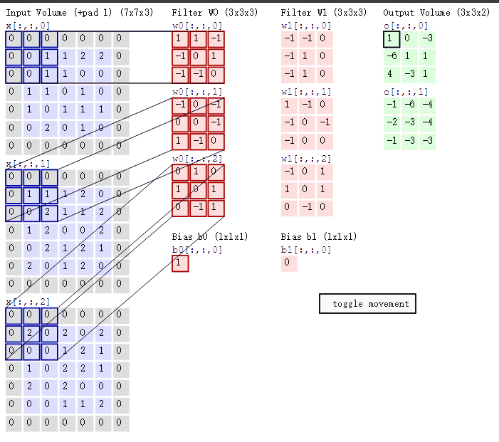
卷积 convolution

对图像（不同的数据窗口数据）和滤波矩阵（一组固定的权重）做矩阵内积（对应元素相乘再求和）的操作就是所谓的“卷积”。

步长stride

即移动的步长

池化pooling

分最大池化、平均池化。作矩阵内积时，分别选取图像对应矩阵中最大值、平均值。就是取区域最大或者区域平均。

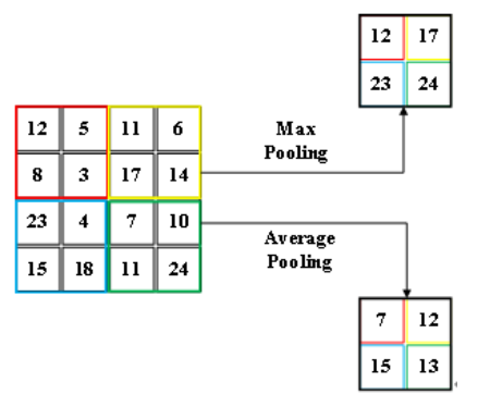
作用：

1. 保留图像的重要特征
2. 数据降维

滤波器filter

即滤波矩阵W0、W1

卷积核Kernel

即W0、W1下的3个红色、粉红色矩阵

补全padding

即为了得到其他维度的结果，周围一圈按情况补0。

channel

即一个图像

4. 一维卷积

卷积核仅沿一个方向移动。

代码示例

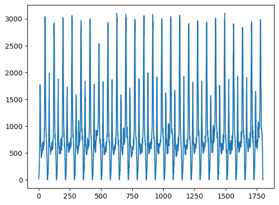
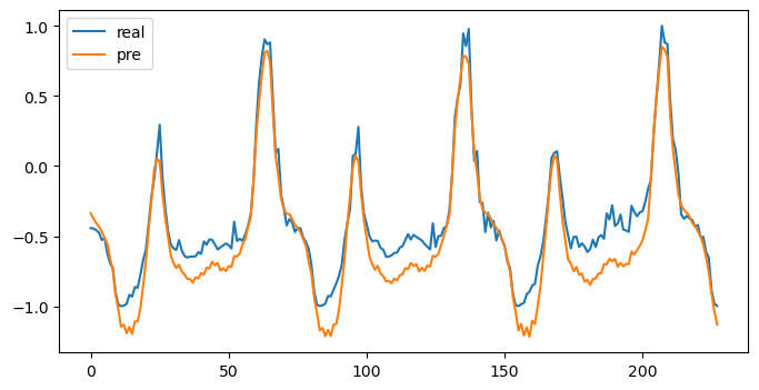
以2016年北京地铁西直门站每15min客流的进站数据为例，利用PyTorch搭建一维卷积神经网络，实现对进站客流数据的预测。

1. 导包

import torch
import torch.nn as nn
import matplotlib.pyplot as plt
import numpy as np
import pandas as pd
from sklearn.preprocessing import MinMaxScaler
from numpy.lib.stride_tricks import sliding_window_view

path = './卷积神经网络/15min_in.csv'
df = pd.read_csv(path, encoding='gbk', parse_dates=True)
data = df['西直门'].values.astype('float32')

plt.plot(data)
plt.show()

​
​

2. 拆分数据集

print(len(data))
split_num = 300
train = data[:-split_num]
test = data[-split_num:]

1800

3. 归一化，按时间窗初始化数据

'''
归一化
'''
scaler = MinMaxScaler(feature_range=(-1,1))
train_norm = scaler.fit_transform(train.reshape(-1,1))
test_norm = scaler.fit_transform(test.reshape(-1,1))
# 转tensor并摊开
train_set = torch.FloatTensor(train_norm).view(-1)
test_set = torch.FloatTensor(test_norm).view(-1)
'''
样本提取（时间窗）
从原时间序列中抽取出训练样本，用第1个值到第72个值作为X输入，预测第73个值作为y输出
'''
Time_window_size = 72
def input_data(seq, ws):  
    out = []
    L = len(seq)
    for i in range(L-ws):
        window = seq[i:i + ws]
        label = seq[i + ws:i + ws + 1]
        out.append((window, label))
    return out
train_data = input_data(train_set, Time_window_size)
test_data = input_data(test_set, Time_window_size)

4. 模型搭建

'''
模型搭建
'''
class CNN_NETWORK(nn.Module):
    def __init__(self):
        super(CNN_NETWORK,self).__init__()
        # 使用64个卷积核，大小为2，在一维序列上进行一维卷积
        self.conv1d = nn.Conv1d(in_channels=1, out_channels=64, kernel_size=2)
        # 激活函数：为卷积输出引入非线性
        self.relu = nn.ReLU(inplace=True)
        # 使用32个卷积核，大小为2，在64维序列上进行一维卷积
        self.conv1d2 = nn.Conv1d(in_channels=64, out_channels=32, kernel_size=2)
        # 一维最大池化层，窗口大小 2、步幅 2，将时序长度缩减一半，突出最显著特征并降低计算量。
        self.pool = nn.MaxPool1d(kernel_size=2, stride=2)
        self.fc1 = nn.Linear(32*35, 640)
        self.fc2 = nn.Linear(640, 1)
        # Dropout 层，训练时随机丢弃 50% 的神经元，防止过拟合。
        self.drop = nn.Dropout(0.5)
    
    def forward(self,x):
        '''
        x [1,1,72] -> [1,64,71]
        input N(batch) Cin(seq) Lin(size) 
        '''
        x = self.conv1d(x) 
        # 激活函数，shape不变
        x = self.relu(x)
        '''
        x [1,64,71] -> [1,32,70]
        '''
        x = self.conv1d2(x)
        x = self.relu(x)
        '''
        x [1,32,70] -> [1,32,35]
        '''
        x = self.pool(x)
        x = self.drop(x)
        '''
        x [1,32,35] -> [1120]
        '''
        x = x.view(-1)
        '''
        x [1120] -> 640
        '''
        x = self.fc1(x)
        x = self.relu(x)
        '''
        x [1120] -> 640
        '''
        x = self.fc2(x)
        return x

device = torch.device("cuda")
net = CNN_NETWORK().to(device)
print(device)

cuda

5. 模型训练

'''
模型训练
'''
criterion = nn.MSELoss()
optimizer = torch.optim.Adam(net.parameters(), lr=0.0005)

epoch = 2

for e in range(epoch):
    for seq, y_train in train_data:
        optimizer.zero_grad()
        y_train = y_train.to(device)
        seq = seq.reshape(1,1,-1).to(device)
        y_pre = net(seq)
        loss_val = criterion(y_pre,y_train)
        loss_val.backward()
        optimizer.step()
    print(f'epoch:{e},loss:{loss_val}')

epoch:0,loss:0.00025611836463212967
epoch:1,loss:0.03752532973885536

6. 画图

test_seq = torch.FloatTensor(test)
realVal = []
preVal = []
with torch.no_grad():
    net.eval()

    for seq, y_test in test_data:
        seq = seq.reshape(1, 1, -1).to(device)
        test_pre = net(seq)
        realVal.append(y_test.numpy())
        # 注意要把cuda变量扔回cpu
        preVal.append(test_pre.cpu().numpy())

plt.figure(figsize=(8,4))
plt.plot(realVal, label='real')
plt.plot(preVal, label='pre')
plt.legend()
plt.show()

5. 二维卷积

卷积核仅沿2个方向移动。

代码示例

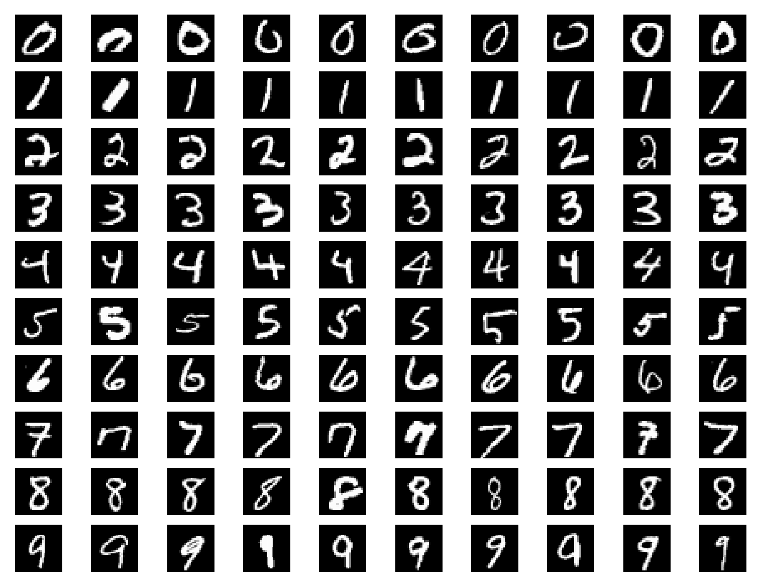
使用PyTorch搭建二维卷积神经网络，用来识别MNIST手写数字数据集，对手写数字进行分类。

transforms.Compose([...])

这是一个组合多个变换操作的容器。这里的操作会按顺序依次作用在输入的图像上。

MNIST数据集包含了60000个训练集和10000个测试数据集，分为图片和标签。图片是28×28的像素矩阵，每张图片是一个手写数字（0 到 9 之间）。标签为0~9共10个数字。

1. 初始化数据

import matplotlib.pyplot as plt
import numpy as np
import torch
import torch.nn as nn
from PIL import Image
import torchvision
import torchvision.transforms as transforms
import torch.utils.data as Data
import torch.optim as optim

def getDataLoader(is_train):
    batch_size = 512
    tra = transforms.Compose([
        transforms.ToTensor(), # 把图像转为Tensor
        transforms.Normalize(mean=[0.5], std=[0.5]) # 归一化
    ])
    dataset = torchvision.datasets.MNIST(root='./卷积神经网络/Datasets/MNIST', train=is_train, transform=tra,download=False)
    # num_workers = 0表示不需要多线程工作
    loader = Data.DataLoader(dataset,batch_size=batch_size,shuffle=True, num_workers=2)
    return loader

train_loader = getDataLoader(True)
test_loader = getDataLoader(False)

2. 初始化模型

# 卷积层
class Conv2dModule(nn.Module):
    # def __init__(self):
    #     super(Conv2dModule,self).__init__()
    #     self.conv2d = nn.Sequential(
    #         # 第一层
    #         nn.Conv2d(in_channels=1, out_channels=32, kernel_size=3,stride=1, padding=1),
    #         # 从每个局部区域中提取最大值，从而降低特征图尺寸，保留主要特征，减少计算。
    #         nn.MaxPool2d(kernel_size=2, stride=2),
    #         nn.ReLU(inplace=True),

    #         # 第二层
    #         nn.Conv2d(in_channels=32, out_channels=64, kernel_size=3,stride=1, padding=1),
    #         nn.MaxPool2d(kernel_size=2, stride=2),
    #         nn.ReLU(inplace=True),
    #     )
    #     self.relu = nn.ReLU()

    def __init__(self):
        super(Conv2dModule,self).__init__()
        self.Conv2d_1 = nn.Conv2d(in_channels=1, out_channels=32, kernel_size=3,stride=1, padding=1)
        self.MaxPool2d = nn.MaxPool2d(kernel_size=2, stride=2)
        self.ReLU = nn.ReLU(inplace=True)
        self.Conv2d_2 = nn.Conv2d(in_channels=32, out_channels=64, kernel_size=3,stride=1, padding=1)
        self.fc1 = nn.Linear(64*14*14, 1024)
        self.fc2 = nn.Linear(1024, 512)
        self.fc3 = nn.Linear(512, num_classes)
        self.num = 1
    
    def forward(self,x):
        # 64 1 28 28 -> 64 32 28 28
        x = self.Conv2d_1(x)
        # 64 32 28 28 -> 64 32 14 14
        x = self.ReLU(x)
        # 64 32 14 14 -> 64 64 14 14
        x = self.Conv2d_2(x)
        # 64 64 14 14 -> 64 64 7 7 
        x = self.MaxPool2d(x)
        x = self.ReLU(x)

        x = x.view(-1,64*14*14)
        x = self.fc1(x)
        x = self.ReLU(x)
        x = self.fc2(x)
        x = self.ReLU(x)
        x = self.fc3(x)
        self.num +=1
        return x

3. 编写训练和测试函数

lr = 0.001
device = torch.device('cuda' if torch.cuda.is_available() else 'cpu')
num_classes = 10 # 共有十种类别的数据图像

net = Conv2dModule().to(device)
criterion = nn.CrossEntropyLoss() # 交叉熵损失函数
optimizer = optim.Adam(net.parameters(), lr=lr)

def getCudaData(tensor,device):
    return tensor.to(device).float()

def train_fn(dataloader,net,device):
    '''
    返回整个过程的平均损失和模型准确率
    '''
    loss_sum = 0 # 损失函数值（总共）
    correct_num = 0 # 预测与真实相符的数量
    sample_num = 0 # 样本数量
    batch_sum = len(dataloader)
    net.train()
    for batch_id,(inputs,labels) in enumerate(dataloader):
        optimizer.zero_grad()
        inputs = getCudaData(inputs,device).float()
        # 交叉熵函数只对类型long支持
        labels = getCudaData(labels,device).long()
        print(f'inputs shape:{inputs.shape}')

        labels_pre = net(inputs)
        loss = criterion(labels_pre, labels)
        
        loss.backward()
        optimizer.step()

        loss_sum += loss.item()
        # 找出样本值里最大idx，定为预测值
        pre_index = torch.argmax(labels_pre, dim=1)
        correct_num += (pre_index == labels).sum().item()
        sample_num += len(labels)

    loss_avg = loss_sum / batch_sum
    correct_rate = correct_num / sample_num

    return loss_avg, correct_rate

def test_fn(dataloader,net,device):
    '''
    返回整个过程的平均损失和模型准确率
    '''
    loss_sum = 0 # 损失函数值（总共）
    correct_num = 0 # 预测与真实相符的数量
    sample_num = 0 # 样本数量
    batch_sum = len(dataloader)
    
    with torch.no_grad():
        net.eval()
        for batch_id,(inputs, labels) in enumerate(dataloader):
            inputs = getCudaData(inputs, device).float()
            labels = getCudaData(labels, device).long()

            labels_pre = net(inputs)
            loss = criterion(labels_pre, labels)
            loss_sum += loss.item()
            
            pre_index = torch.argmax(labels_pre, dim=1)
            correct_num += (pre_index == labels).sum().item()

            sample_num += len(labels)
            
    loss_avg = loss_sum / batch_sum
    correct_rate = correct_num / sample_num
        
    return loss_avg, correct_rate

4. 训练

train_loss_list = []
test_loss_list = []
train_cro_rate_list = []
test_cro_rate_list = []

epoch = 10
for e in range(epoch):
    train_loss, train_cro_rate= train_fn(train_loader,net,device)
    train_loss_list.append(train_loss)
    train_cro_rate_list.append(train_cro_rate)

    test_loss, test_cro_rate= test_fn(test_loader,net,device)
    test_loss_list.append(test_loss)
    test_cro_rate_list.append(test_cro_rate)

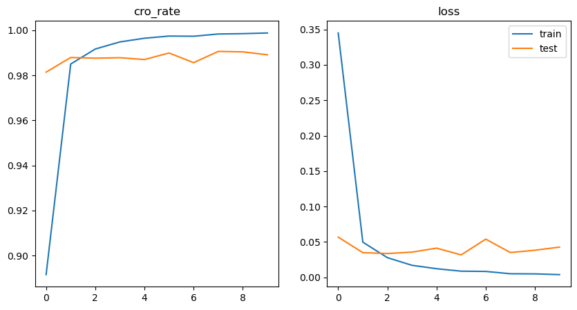
5. 画图

fig = plt.figure(figsize=(10,5))
ax1 = fig.add_subplot(1,2,1)
ax1.plot(train_cro_rate_list, label='train')
ax1.plot(test_cro_rate_list, label='test')
ax1.set('cro_rate')

ax2 = fig.add_subplot(1,2,2)
ax2.plot(train_loss_list, label='train')
ax2.plot(test_loss_list, label='test')
ax2.title('loss')
plt.legend()
plt.show()